The binomial distribution is a discrete probability distribution that models the number of successes in a fixed number of independent trials, where each trial has only two possible outcomes:

1. Success (with probability p)
2. Failure (with probability 1 – p)

It is commonly used in situations like flipping coins, quality control in manufacturing, and medical trials.

1. Conditions for a Binomial Distribution

A random experiment follows a binomial distribution if:

1. Fixed Number of Trials (n) – The experiment is repeated n times.
2. Independent Trials – The outcome of one trial does not affect the others.
3. Two Possible Outcomes – Each trial has only two results (Success or Failure).
4. Constant Probability (p) – The probability of success remains the same for all trials.

📌 Example:
A company produces light bulbs, and each bulb has a 5% chance of being defective. If we inspect 10 bulbs, we can model the number of defective bulbs using a binomial distribution with:

• n = 10 (fixed number of trials)
• p = 0.05 (probability of defect)

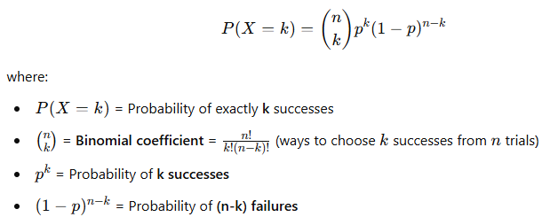
2. Binomial Probability Formula

The probability of getting exactly k successes in n trials is given by:

📌 Example:
If we toss a coin 4 times and want to find the probability of getting exactly 2 heads, we use:

• n = 4
• k = 2
• p = 0.5 (since heads has a 50% chance)

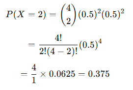
Thus, the probability of getting exactly 2 heads in 4 coin tosses is 0.375 (or 37.5%).

3. Mean and Variance of a Binomial Distribution

For a binomial distribution:

• Mean ($\mu$) = np
• Variance (σ^2) = np(1−p)
• Standard Deviation ($\sigma$) = [np(1−p)]^0.5​

📌 Example:
If a multiple-choice test has 20 questions, and each question has 4 choices (one correct), then:

• n = 20
• p = 1/4 = 0.25 (since each question has a 25% chance of being correct)
• $5$ → Expected correct answers
• σ= [20×0.25×0.75] ^0.5 = 3.75^0.5  ≈ 1.94

This means a student who guesses randomly can expect to get about 5 correct answers with a standard deviation of ~1.94.

4. Shape of a Binomial Distribution

• Symmetric if p = 0.5 (equal success/failure chance)
• Skewed Right if p < 0.5 (success is rare)
• Skewed Left if p > 0.5 (success is common)

📌 Example:

• If we flip a fair coin 10 times, the distribution is symmetrical.
• If we roll a die and count how often we get a 6, the distribution is right-skewed (since getting a 6 is rare: p=1/6​).

5. Applications of Binomial Distribution

✅ Manufacturing – Defective vs. non-defective products
✅ Medical Trials – Success rate of a new drug
✅ Marketing – Probability of customers responding to an ad
✅ Sports – Free throw success in basketball
✅ Finance – Probability of stock price increasing on a given day

Conclusion

• Binomial distribution is useful for modeling “success/failure” experiments.
• It requires a fixed number of independent trials with a constant success probability.
• The probability formula helps determine the likelihood of getting a specific number of successes.
• The mean and variance describe the expected outcomes over many trials.